1. Table of Contents
- The feasibility of quantization and SQ on SparseConv3d: ✅
- The discussion of sparse conv3d:
- Find where the computation for sparse conv3d is done: ✅
- Inside
ops.implicit_gemm: ✅
- How can we implement it:
- Quantization of the activation and weight: ✅
- Application of SQ during quantization process: ✅
- Evaluation of current method:
- Whether SQ is effective or not depends on the value of the inputs and weight: ✅
- Actual implementation: In progress…
2.1 Find where the computation for sparse conv3d is done.
Firstly I went through the source code of spconv (except for CUDA kernel part), and I found out how the computation for sparse conv3d is done:
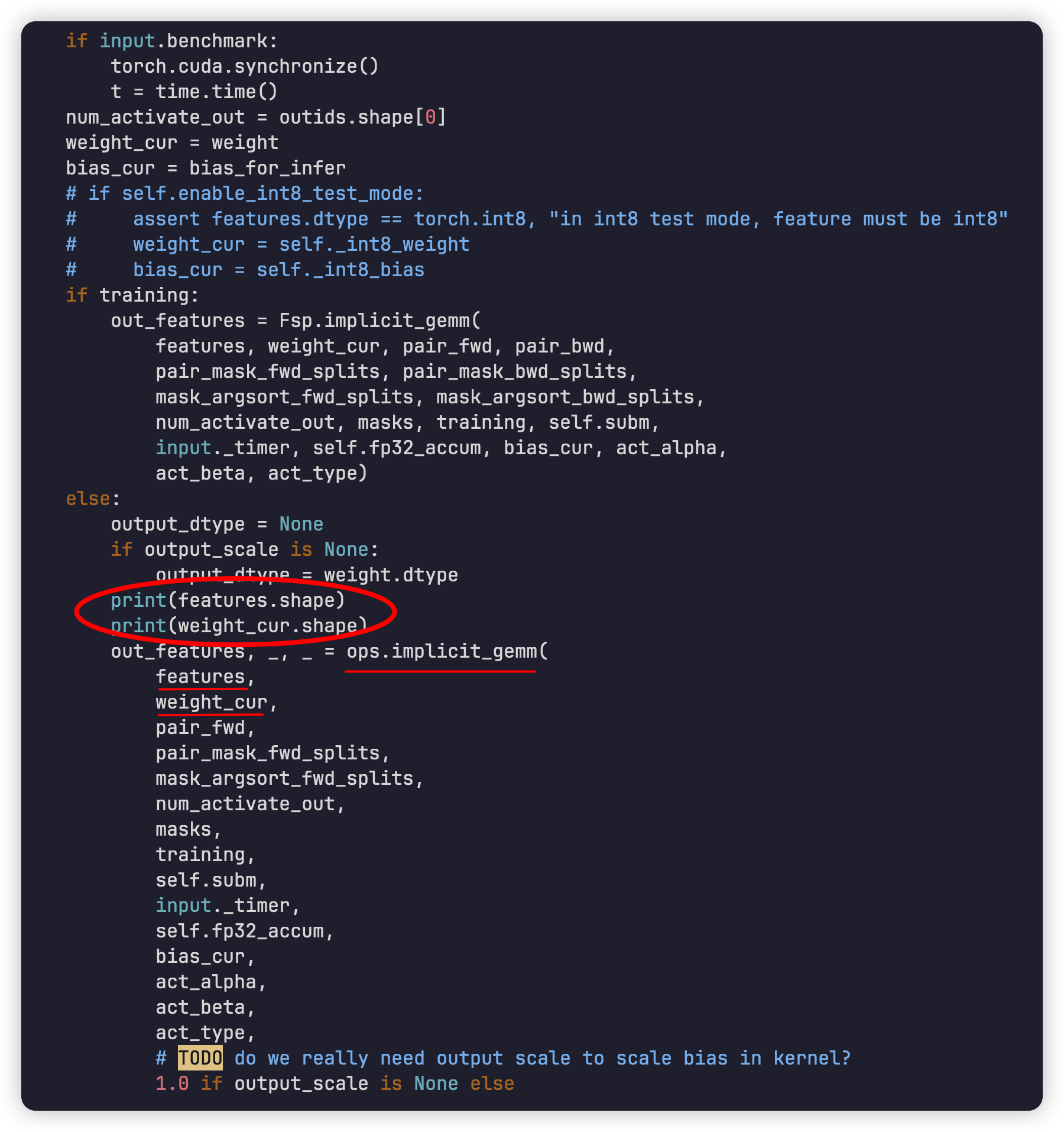
After some preprocessing, we got features and weight_cur.
From the graph, I found that features and weight_cur are then passed into ops.implicit_gemm, so I then print them to find what type they are, which turns out that both of them are Tensor. I then print out the shape and the results are similar to the following:
feature.shape: torch.Size([124310, 5])
weight_cur.shape: torch.Size([16, 3, 3, 3, 5])
Here, what I think that makes it a little difficult is that the shape of the feature is indeed a 2d matrix, but the shape of the weight is just a standard shape for Conv3d, which makes the gemm process of feature and weight not that intuitive for me. So I then looked into ops.implicit_gemm to see if there’s any hope.
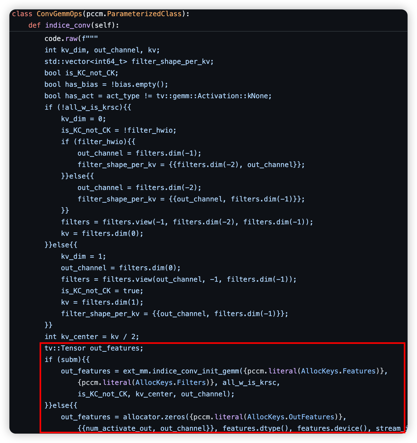
2.2 Inside ops.implicit_gemm
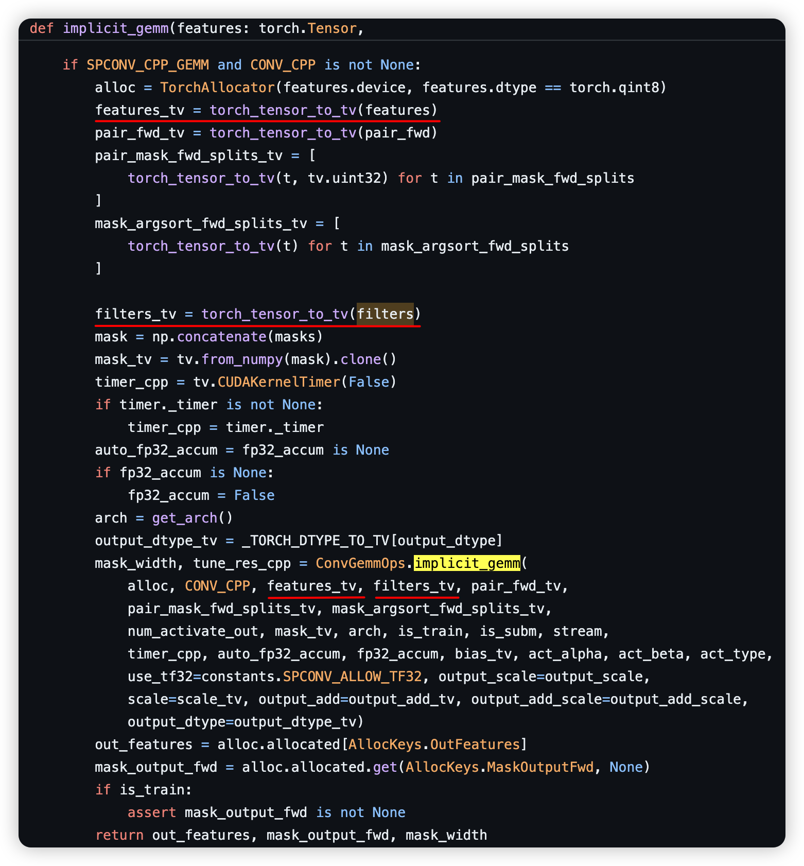
Inside ops.implicit_gemm, both features and weight are cast to a data type tensorview, which is commonly utilized in cumm, a python asyncio-based gemm simulator written by the creator of spconv package. After the transformation of the data type, both of them are passed into ConvGemmOps.implicit_gemm, which is as follow, utilizing pccm (which needs some c or cuda), another package written by the creator of spconv, to achieve the computation of the out_features (inside red box below, this picture is wrong, will change it in the future):
3.1 Quantization of the activation and weight
There’s actually an equivalent logic here if we want to quantize the activation and weight of the spconv3d layer under one specific hypothesis:
If the outcome of
spconv3dandconv3dare the same.
It turns out that this is true, and therefore, we can start working on the quantization of both activation and weight:
-
For activation: Since we only apply per-tensor quantization to the activation, we just need to get the element that has the max absolute value of the whole activation tensor to apply quantization.
-
For weight: Since the weight for sparse 3d convolutional and normal 3d convolution is the same, per-channel quantization should be similar without difficulty.
3.2 Application of SmoothQuant during quantization process
If we want to apply SmoothQuant to our quantization as well, we need an extra hypothesis below:
If the computation of
spconv3dcan be transformed into img2col + gemm format.
And it turns out that the img2col process is just similar to the normal 2d unfold process, but instead we unfold three times on three different dimensions.
Hence, we can actually first convert the input/activationof the spconv3d layer into dense format, transform it into a 2d matrix format using img2col and get the max list similar to the 2d process. The part for the weight is also similar, we unfold it into a 2d matrix format, and then get the max list. After getting two lists, we can compute the scale list and scale the magnitude of activation down while scaling up the weight to migrate the quantization difficulty from activation to weight.
4.1 Evaluation of current method
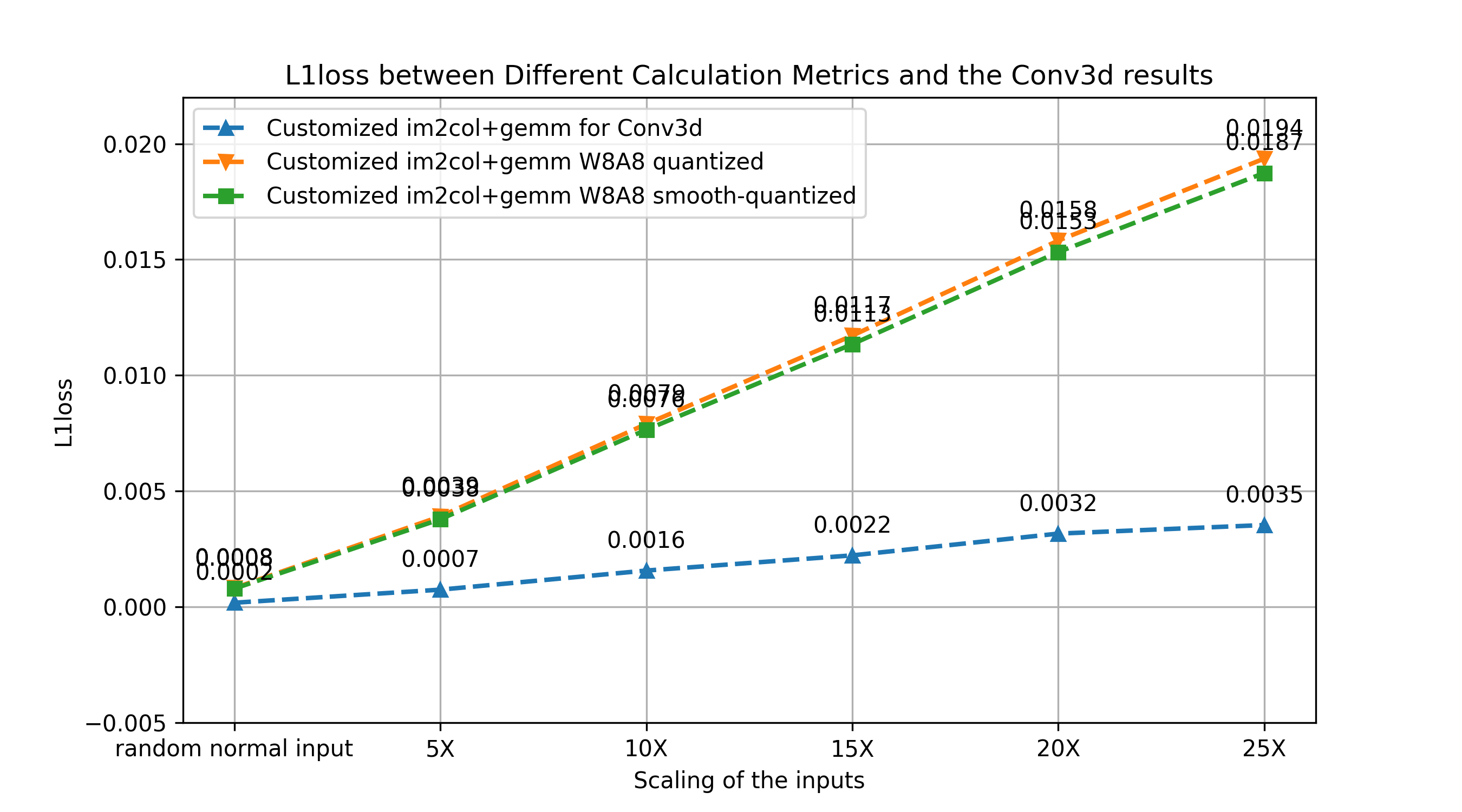
Here, the x-axis are the same random normal inputs with different scaling, while y-axis is the L1 Loss between the method that the line represents and the original Pytorch conv3d implementation.
We can get a conclusion from the graph, which is: whether SQ is effective or not depends on the value of the inputs and weight. We can also witness greater loss within the blue line, which means that further improvement for the current method is needed.
4.2 Evaluation with different scaling factor
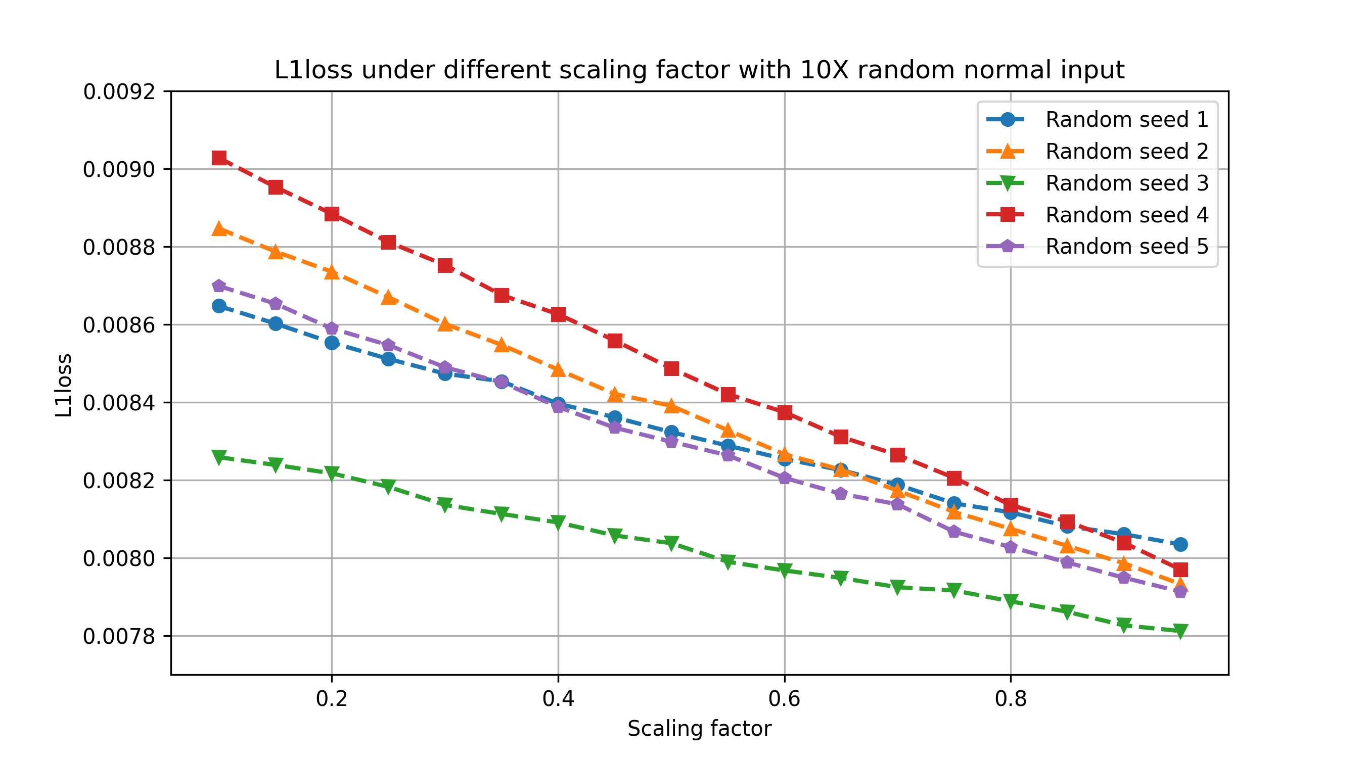
Here, the x-axis are different random normal inputs with different scaling factor (from SmoothQuant), while y-axis is the L1 Loss between our method and original Pytorch conv3d implementation with specific example 10X inputs. From the graph, we may guess that our method is effectively dealing with the quantization difficulty from the activation.
5. What’s next?
- Apply naive W8A8 quantization to Centerpoint:
- check the accuracy:
- If accuracy doesn’t drop much, maybe there’s no need of SmoothQuant.
- If drops much, focusing on how to apply SmoothQuant to spconv3d after quantization.
- check the accuracy:
- Check the baseline of my method:
- Figure out why there’s greater loss along with the scaling of the example inputs without any quantization, and try to fix it.
- Check the activation outlier:
- After going through the above first two points, we can check the activation to see where the outliers are if they indeed exist.
- Expand on the data structure of SparseConvTensor on our next meeting with clearer explanation.